Flower Bud Formation Revisited
Mark P. Widrlechner
Ames, Iowa
I read with great interest Dr. Russell Gilkey's article in the Winter 1996 issue of the Journal concerning relationships among factors that may have influenced the development of rhododendron flower buds in his garden (1). Dr. Gilkey's perseverance in amassing so much valuable information is remarkable. His data set, compiled over 18 years, can be used to develop testable hypotheses about flower bud formation that may help other gardeners predict or manipulate future floral displays.
Multiple-regression analysis is a statistical tool that allows us to construct predictive models that involve multiple factors of the sort that Dr. Gilkey reported. More specifically, such models are concerned with the problem of describing or estimating the value of one factor (called by statisticians, the "dependent variable") on the basis of one or more other factors (called "explanatory variables"). Multiple-regression models thus take the form of mathematical equations that give an estimate of one factor we wish to study based on functions that weight the contributions of other factors.
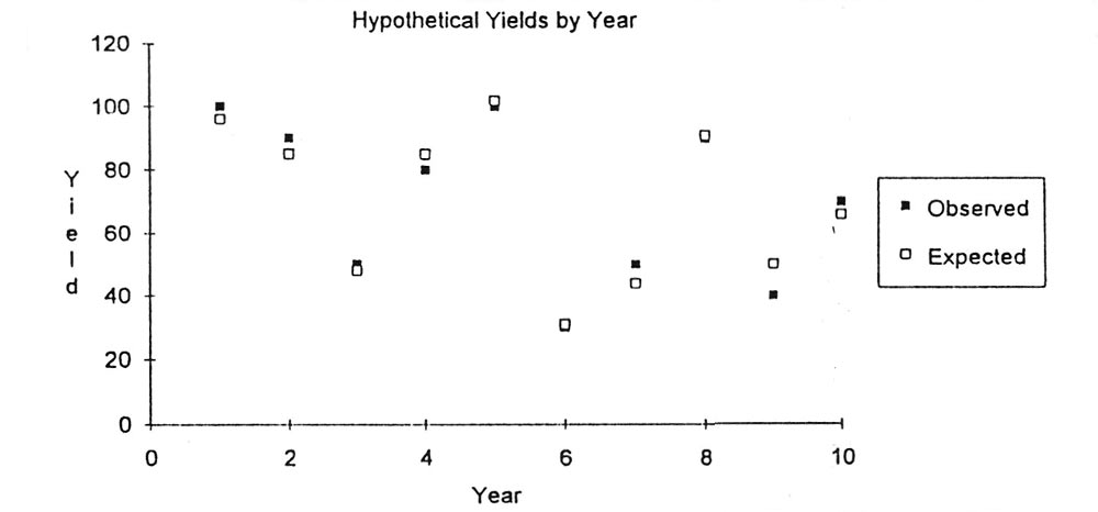
As a hypothetical example, let us say that a truck farmer had grown 'Rutgers' tomatoes for 10 years in a row and recorded the yields each year (Table 1). The yields varied widely from year to year (Figure 1). What might explain this variation? The farmer suspects that July temperature, length of the growing season, and disease severity could have all played roles, so values for these factors were collected as well (Table 1). Multiple-regression analyses test simple mathematical equations combining these factors to identify an equation that best predicts the year-to-year variation in yield. For this hypothetical situation, the best predictor of yield was the equation: Yield = (1.71 times July temperature ) + (0.63 times growing season) - (3.93 times disease severity) - the constant, 104.3, known as the intercept.
| Table 1. Hypothetical Tomato Yields | ||||
| Year | Yield | July Temp. | Growing Season | Disease Severity |
| 1 | 100 | 80 | 120 | 3 |
| 2 | 90 | 75 | 110 | 2 |
| 3 | 50 | 70 | 90 | 6 |
| 4 | 80 | 80 | 90 | 1 |
| 5 | 100 | 85 | 110 | 2 |
| 6 | 30 | 65 | 100 | 10 |
| 7 | 50 | 65 | 90 | 5 |
| 8 | 90 | 80 | 100 | 1 |
| 9 | 40 | 65 | 100 | 5 |
| 10 | 70 | 75 | 80 | 2 |
|
| Figure 1 |
In other words, an increase in one degree in July temperature was associated with an increase of 1.71 in yield; an increase of one day in the growing season was associated with an increase of 0.63 in yield; and an increase of one unit of disease severity was associated with a decrease of 3.93 in yield. Figure 1 shows how well this equation was correlated with yield. Over 95% of the year-to-year variation in yield was explained by this particular model. Since this technique can weigh and combine relationships among different factors, I was curious to learn whether multiple-regression analysis could shed additional insight into the control of rhododendron flower bud set.
Thus I decided to re-analyze Dr. Gilkey's data by using software designed to perform correlation and multiple-regression analyses (2). First, I developed a table with 10 variables for a period of 17 years, 1978 to 1994. These variables were:
V1 - Flower buds per plant
V2 - Last year's flower buds per plant
V3 - Bud change index
V4 - Blast
V5 - Fertilizer
V6 - Moisture deviation
V7 - Cooling degree day deviation
V8 - Non-cloudy day deviation
V9 - May mean temperature
V10 - Mean plant age.
The variables were calculated as follows. V1 was simply "Total No. Buds" divided by a modification of "No. Plants Counted" from Dr. Gilkey's Table 1 (1). Dr. Gilkey informed me that "No. Plants Counted" did not include plants counted for the first time in a given year, so these new plants were added to "No. Plants Counted." V2 was V1 from the previous year. V3 was the "No. Plants Whose Buds Increased" minus the "No. Plants Whose Buds Decreased," all divided by the unmodified "No. Plants Counted," from Table 1. V1 and V2 standardized the data on a per plant basis, allowing for year-to-year comparisons. And V3 created a single variable to examine the net change in the number of buds among many plants. V4 was coded as 1 in 1982, 1984, 1985, and 1994, and as 0 in the other years. V5 was coded as 1 in 1990, 1991, 1993, and 1994, and as 0 in the other years. V6 was coded from Dr. Gilkey's Table 2 as "June, July, August Rainfall" for 1978 to 1983, and as "June, July, August Irrigation Plus Rainfall" after 1983 (1). V7, V8, and V9 were entered directly from the last three columns of Table 2. V10 comprised unpublished data that I obtained from Dr. Gilkey (personal communication) because I suspected that plant maturity could have a role in bud production. Mean plant age varied between 11.2 and 14.5 years during the study period.
Statistical models to predict flowering from these data need to examine how factors might explain variation in V1, the number of flower buds per plant, and V3, the bud change index, a measure of the strength of bud-set increase or decrease among plants for any given year. Once the table was entered and proofed, I first performed a series of pair-wise correlations, to see if any single factor might determine V1 and/or V3. For V1 (flower buds per plant), only V3 and V4 were significantly correlated. For V3 (bud change index), only V1, V2, and V9 were significantly correlated. One would expect a correlation between V1 and V3, almost by definition, because the number of flower buds per plant is a function of last year's number and the bud change index.
So all I could really say from simple correlations was that flower buds per plant were positively correlated with blast and that the bud change index was positively correlated with May mean temperature and negatively correlated with last year's flower buds per plant. Although these three correlations were statistically significant, they each only explained between 26% and 55% of the year-to-year variation in flower buds per plant or in the bud change index.
This lack of predictive power was not very satisfying, so I proceeded to test models involving combinations of multiple, linear factors by using multiple-regression analysis. The results were enlightening, because the best models were highly statistically significant and they explained more of the total variation than did any of the previous correlations. For V1 (flower buds per plant), the best regression model was:
2. V1 = 22.6 V4 + 2.91 V9 + 6.84 V10-47.96. This model basically states that the number of flower buds per plant is a linear function of blast, May mean temperature, and mean plant age. Here a "blast year" is associated with an increase of 22.6 flower buds per plant, an increase of one degree in May mean temperature is associated with an increase of 2.91 flower buds per plant, and a year of plant maturity is associated with an increase of 6.84 flower buds per plant. It explained 72% of the total variation in the number of flower buds per plant and was significant at the 0.001 level. The statistical significance of this model could not be improved by adding any other variables to it.
Turning to V3, the bud change index, the best regression model was:
3. V3 = -0.016 V2 + 0.34 V4 + 0.043 V9 + 0.73.
In other words, last year's flower buds per plant, blast, and May mean temperature all influenced the bud change index. This model explained 71 % of the variation in the bud change index and was significant at the 0.001 level.
From these models and many other inferior models that I tested, I would conclude that last year's flower buds per plant, blast, plant age and May mean temperatures were much more important than were fertilization, summer moisture levels, or summer temperatures in determining the flower bud set in Dr. Gilkey's garden. The roles of last year's bud set, blast, and plant age are straightforward. But why did May temperatures work and not the summer climatic variables? I suspect that in Kingsport, Tenn., the energy gained by rhododendrons during May might shift development from vegetative to floral meristems, which could place buds on a developmental path that summer stresses could only slightly alter under normal circumstances.
Dr. Gilkey indicated that there were "non-conforming" years, such as 1991, that were hard to explain (1). There is a statistical technique that can be used to identify "non-conforming" years. A residual is the difference between what was observed and what was predicted by a statistical model. (In Figure 1, the residuals are measured by the differences between the observed and the predicted points.) Residuals can be standardized to search for such "non-conforming" years. When I analyzed residuals for my models 2 and 3, I found no examples of statistically "non-conforming" years. Model 2 had the poorest prediction of the number of buds per plant for 1987 and model 3 had the poorest prediction of bud change index for 1980. But for both years the residuals were still within normal expectations.
In summary, multiple-regression analyses can be employed to identify relationships among many, independent factors that together could influence some final outcome. A re-analysis of Dr. Gilkey's (1) flower bud and climatic data suggests that last year's flowering, bud blast, plant age, and May mean temperatures are important factors together influencing the floral display in his garden and perhaps in many other gardens in his region.
The multiple-regression equations that I tested were all linear equations, ignoring any complex interactions among factors. If there are significant interactions among climatic variables, or if relationships between factors and bud set are really not linear, other, more refined models could be even better predictors of flower buds per plant and the bud change index.
I hope that Dr. Gilkey's diligence in collecting such a valuable data set will inspire other members to document similar phenomena in their gardens. Important topics to examine would include determining whether there are critical times of the year when the temperature most influences bud set under local conditions and whether bud removal in particularly floriferous years might reduce year-to-year fluctuations.
Acknowledgments
Ideas resulting from critiques by Sharon Dragula and Richard Schaefer were very helpful. And I am especially grateful to Russell Gilkey for kindly sharing so much valuable information with me.
References
1. Gilkey, R. Correlation between weather conditions and rhododendron flower bud formation. J. Amer. Rhod. Soc. 50:38-40; 1996.
2. Nissen, O.; Everson, E.H.; Eisensmith, S.P.; Smail, V.; Anderson, J.; Rorick, K.; Portice, G.; Rittersdorf, D; Wolberg, P.; Weber, M.; Freed, R.; Bricker, B.; Heath, T.; Tohme, J. MSTAT - A microcomputer program for the design, management, and analysis of agronomic research experiments (Version 4.0). Michigan State Univ., East Lansing, and Agric. Univ. of Norway, Aas.; 1985
Dr. Widrlechner is the Horticulturist of the North Central Regional Plant Introduction Station, USDA, and a member of the ARS Research Committee.