JOTS v27n2 - Software to Simulate and Optimize Asset Management in Constuction and Manufacturing

Software to Simulate and Optimize Asset Management in Construction and Manufacturing

M.D. Salim	Marc A. Timmerman

In the 21st century asset management and resource allocation will be key technologies for the successful management of many public and private enterprises. In teaching asset management techniques in construction management and manufacturing courses in industrial technology programs, there is a challenge of finding enhancements to textbook-based instruction. Software tools to simulate realworld style problems in asset management are a valuable enhancement to this classical style of pedagogy. This article describes a number of such currently available tools. It also evaluates them according to such factors as cost, ability to solve complex problems, and suitability for use by nonspecialist students. The issue of using such tools to teach optimization techniques for asset management in the classroom setting using artificial intelligence methods of optimization is also explored. Finally, an overview of a real-world asset management case study as an instructional concept for classroom use is presented.

What Is Asset Management?

Asset management combines and integrates the acquisition, evaluation, storage, and distribution of assets and resources required by an organization. A tremendous amount of management control can be exerted through a properly designed asset management and resource allocation system that is operated by trained management personnel. But, there are costs involved with developing and implementing an asset management system. Organizations using such systems must dedicate resources for funding their implementation. The costs and benefits of asset management systems vary greatly, depending on the type of systems implemented, the scope of the systems put into service, and a number of other factors. Rapid changes in existing technologies require frequent updating of asset management systems. In many cases, the changes are so significant that completely new systems must be developed.

Figure 1
Asset and Resource Management Paradigm.

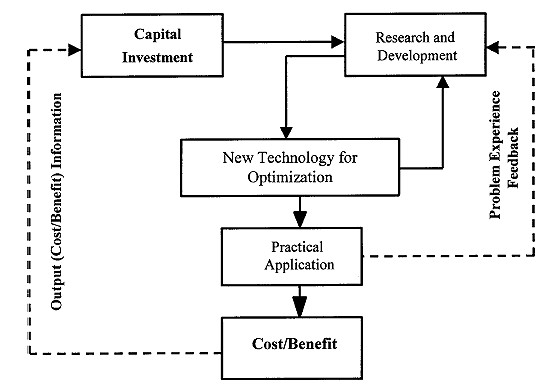
Capital investment is the key stimulus for updating existing and developing a new asset management system as indicated in Figure 1. Capital investment enables research and development, which leads to improved technology for asset management and resource allocation. The figure also suggests that cost/ benefit analysis on the practical applications of this improved technology is usually relevant. A computer-based asset management system will track what equipment and other resources are to be issued for a specific project including personnel composition and personnel assignments. Studies have shown that personnel are much more productive when an asset management system tracks assets and other allocated resources in real-time.

The recent literature on the importance of asset management to construction, manufacturing, and other industrial technology education areas is enormous. Some highlights would include the work of Satter, Wood, and Ortiz ( 1998 ) on the use of asset management in petroleum industry related construction. Curtis and Molnar ( 1997 ) have described the use of asset management in public works construction. Carpenter ( 1997 ) has written about the use of asset management in manufacturing, specifically in the area of machining. Gibson ( 1998 ) and Van Rijn ( 2000 ) have described the use of asset management tools for the maintenance aspects of manufacturing. Finally Stys ( 1997 ) has written about the use of asset management for maintenance in the utility industry.

Artificial Intelligence

Authors define artificial intelligence (AI) in different ways. For example, Kurzweil ( 1990 ) defined AI as the art of creating machines that perform functions that require intelligence when performed by people. According to Lugar and Stubblefield ( 1993 ), AI is the branch of computer science that is concerned with the automation of intelligent behavior. In the past decade there have been numerous articles about the application of AI as "expert systems," which are also called "knowledge-based systems" by some investigators.

Figure 2
Artificial Intelligence Concepts.

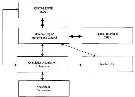
The architecture of an expert system is presented in Figure 2. It shows that knowledge engineering is the first step in creating an expert system. The knowledge engineer usually acquires and places the knowledge into the expert system's knowledge base. In other words, the knowledge engineer is the interface between the human expert and the expert system. In an expert system the knowledge base is kept separate from the control mechanism known as the inference engine, which directs or controls the system when it searches its knowledge base in a dynamic environment. The expert system can be integrated with other programs and/or databases to solve specific problems. In the following paragraphs, we describe a model of an expert system to optimize asset management. It is an AI-based system that uses a Geographic Information System (GIS) database for attributes and values to optimize asset/resource management.

Selecting an Artificial Intelligence Shell

A computer software that is very often utilized for the development of an expert system is known as an "AI shell." These AI shells are generic software environments to implement expert systems, much in the same way as a word processor is a software environment to edit text. However, selection of the correct shell to meet specific needs is becoming increasingly critical, considering the ever-growing use of computers and the availability of diverse shells to build expert systems. The fundamental issues of choosing "shells" for asset/resource management applications are offered beginning with a six-step plan of action for selecting a shell: (1) define the selection criteria; (2) find all available shells that might fit the needs or criteria chosen; (3) narrow the list obtained from the second step down to a revised or a short list; (4) try to shorten the list even more by researching those shells in much greater detail; (5) test the remaining shells; and (6) select and purchase the most suitable shell.

We began our study on available shells with the creation of a list of criteria as in Step 1. These requirements can vary greatly depending on the task and the size of job. It is important to note that selection of shells is always need-driven. We listed the criteria as follows:

• Platform it runs on (Windows, Unix). Windows is preferred for instructional use.
• Limitation on the number of rules. Must have more than 100 rules for planned scope of class projects.
• Limitations on database size. Must be able to use large GIS databases 100 MEG+ for planned class projects.
• Speed of execution. Must be fast enough to be able to run several complex cases in the space of a two-hour lab session.
• Internet interface capabilities. Very desirable in a distributed network environment such as a teaching lab.
• Compatibility with GIS package. Must be able to read data from desired databases for class projects.
• Cost and licensing issues. Must be available in a multi-used academic version at reasonable cost.

Table 1
Commercial AI Shell Packages.
Company	Product	Problems	Price
Neuron Data Systems	Nexpert Object	Costly but Good	$16,000 +
Expertelligence	WebBase ANDE	Limited to number of rules < 50	$495
Intellicorp	PowerModel™ LiveModel™	Poor interface to all databases	$3,129 $3,049
Level 5 Research Inc.	Level 5 Object	Non-generic production language	$5,000+
Neuron Data	Intelligent Rules Element	Costly but Good	$6,000 - $12,000
Micro Data Base Systems	Guru	Costly but Good, some interface issues.	$7,000 (single user) $15,000 (LAN user)
Exsys Professional	EXSYS Professional	Still under evaluation	$5,000
Wordtech Systems	VP Expert	Limited Rules, Small applications only	$349 39.95(educational price)
Art Enterprise Systems	Art * Enterprise	Extensive LISP Programming Needed	$8,000

For Step 2 we considered shells advertised on the Internet and in computer trade magazines and professional journals and periodicals. Because there are literally hundreds of shells that deal with different types of applications and users, this is a daunting tasks. A short list of the shells is created based upon the selection criteria is created under Steps 3 and 4. In the final steps the shells are tested, resulting in the final list presented in Table 1. The ideal result will be the selection of one shell. This may not always be the case because more than one shell may perform the needed tasks. In this case cost becomes the key factor in deciding what shell to select. In this particular case, the final step was to examine demonstration versions of the selected shells.

Optimization

Optimization is the search for better solutions. Many problems in industry have non-unique solutions, and optimization is a systematic way of generating these non-unique solutions and finding the best solution of the set. The term best can refer to cost, time, energy usage, product quality, or some other beneficial quality of interest. A monograph by Traub and Wozniakowski ( 1980 ) summarized optimization techniques. Lau's ( 1986 ) standard reference of optimization techniques expressed them in the form of computer programs. Khan and Hayhurst ( 2000 ) and Suh and Shin ( 1996 ) described the application of optimization techniques to problems in manufacturing in great detail.

Optimization methods can be thought of as falling in two categories: heuristic and non-heuristic. Non-heuristic techniques involve the application of complex mathematical methods from an area of mathematical analysis known as the calculus of variations. These methods include the dynamic programming method of Bellman, the optimal principle of Pontryagin, the time-dependent Lagrange multiplier method, and derivatives of these methods such as the Hamilton-Jacobi-Bellman method; all are described in detail by Bryson and Ho ( 1975 ). These methods require extremely complex calculations and are generally best suited for highly specialized applications such as the design of NASA's space missions and nuclear weapons research. They are pedagogically unsuited for industrial technology education, and they are, in general, too computationally demanding for use in day-to-day industrial problems.

Heuristic optimization methods are based on concepts from AI. They are based on general observations or "rules" about the qualities of an optimal solution. These rules are programmed into the "shell" and are used repeatedly to generate, improve, and test the solution. Heuristic optimization techniques are pedagogically suitable for industrial technology education and are easily studied using computing resources usually found in industrial technology departments. The relative ease of use and simplicity of these rules also make them useful in the solution of day-to-day industrial problems.

A Case Study: Snow Removal Asset Management

Both manufacturing and construction industries have embraced AI techniques to optimize resource allocation, manage assets, and improve productivity. For example, in manufacturing, as fully automated machinery increases in capability, the assignment of individual jobs to such automated machinery becomes very complex. AI-based optimization techniques have been widely deployed to solve such challenging "shop management" manufacturing problems. To study the manufacturing optimization techniques used for these shop management problems, industrial technology students need some familiarity with the type of automated machines involved, the process times of machining tasks, and similar parameters. The same observations hold true for construction management studies.

The deployment of snow plows in a municipality for the purpose of snow removal is our example of a case study of a problem in optimized asset management. The object is to plan routes for the plows so as to remove the most snow using the least amount of resources such as driver time, plows, sand, and salt. The main reason for selecting snow plowing as our case study is that it is very familiar to students in colder climates from daily life and is also familiar to others from television and cinema depictions. Snow plowing contains all of the needed elements of a good case study in a format that is well suited for instruction.

This problem is an enhanced version of a classical textbook problem in optimization called the traveling salesman problem or the TSP. The idea of the TSP is that a salesman has to make a number of sales calls in different cities. He needs to plan a trip that will allow him to visit the largest number of these cities possible in the least amount of time and traveling distance. Burkard, Deineko, and van Dal ( 1998 ) have contributed an excellent summary of solved TSP problems for instructional purposes. The TSP has many applications in real-world industrial problems such as material delivery in manufacturing settings. Chalasani and Motwani ( 1999 ) and Bertsimas, Chervi, and Peterson ( 1995 ) have also described applications of the TSP to real-world industrial problems.

For our purposes let's assume then that an idealized community has one snow plow, a personnel budget of 100 man-hours, and 1,000 tons of road salt. The optimization problem would be to maximize the miles of road plowed, minimize the cost to the city of the work, stay within the available resources, and respect the physical reality of the problem.

Stated mathematically this would mean that we want to make this expression LARGE:

Miles plowed Road 1 + Miles plowed Road 2 + Miles plowed Road 3 and so on for all roads Total miles of road plowed.

To make this expression SMALL:

Man-hours Road 1 x salary rate +Man-hours Road 2 x salary rate +Man-hours Road 3 x salary rate and so on for all roads +Man Hours Deadheading x salary rate + Salt used on Road 1 x salt cost + Salt used on Road 2 x salt cost + Salt used on Road 3 x salt cost and so on for all roads Total cost of plowing.

While obeying the physical realities of the problem:

• Salt on Road 1 = length of Road 1 x needed salt rate
• Time on Road 1 = length of Road 1/maximum plowing rate
• Salt rate Road 1 = function of road surface, snow depth, temp, etc.
• Plow rate Road 1 = function of road surface, snow depth, temp, etc.
• Road 1 connects to Road 3 only.
• Etc

And also while staying within the limits of the available resources:

Man-hours Road 1 +Man-hours Road 2 +Man-hours Road 3 and so on for all roads +Man-hours Deadheading Less than 100 hours.

Figure 3
Asset Management Case Study.

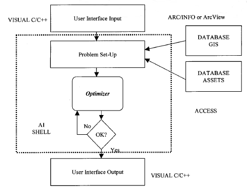
Salt used on Road 1 +Salt used on Road 2 +Salt used on Road 3 and so on for all roads Less than 1,000 tons.

Figure 3 presents an overview of the software tasks that the students would perform in solving this case. The "shell" would be used to implement the heuristic rules to first generate solutions to the problem and then to improve on these solutions. Typically this is done in iterations with the program only stopping when an acceptable solution has been reached. Other tasks would be to write C/C++ programs to format the input and output data in user-friendly forms and to use database software to implement database of the assets involved and of the geography of the city in GIS format.

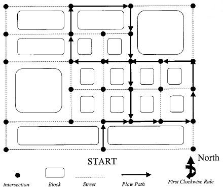
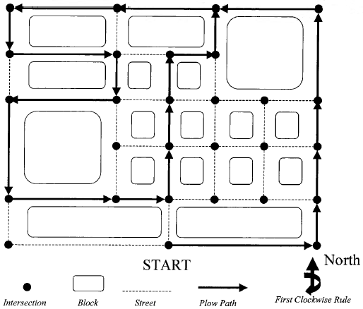
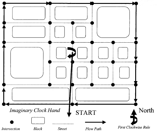
The heuristic rules involved in creating a snow plowing path are quite interesting. In order to generate an optimal solution, a number of heuristic techniques are available. For illustration purposes, a single snowplow is considered as plowing the streets of a small community. Figures 4, 5, and 6 depict the street map. The boxes represent city blocks, the dotted lines represent city streets, and the black circles represent the intersections. The snowplow begins plowing from a fixed starting point. The heuristic rules are presented in terms of this imaginary model.

Figure 4 presents an example of the nearest neighbor heuristic rule. In this rule, the snowplow driver stops at each intersection and picks the shortest street to the next intersection. If there are two or more equally short streets, the plow driver uses the "first clockwise rule." The driver imagines that the minute hand of an imaginary clock is sweeping clockwise from due North at 12 o'clock. The first of the two or more equally short streets to be swept over by the minute hand of this imaginary clock is selected by the driver. As can be seen in the diagram, this heuristic rule results in a relatively short and efficient path, but creates the situation of the same streets being plowed more than once. In contrast, Figure 5 presents the furthest neighbor heuristic rule. In this case the plow driver stops at each intersection and picks the longest street to the next intersection. Again, the driver uses the first clockwise rule to select from two or more equally long streets. This heuristic rule creates a much longer and more winding path than the nearest neighbor heuristic rule. This path also requires some streets to be plowed more than once. Figure 6 presents the circular route heuristic rule. In this rule the driver creates a mental picture of an imaginary clock whose minute hand is centered at the geographic center of the city. The driver imagines the minute hand of this clock sweeping over the plow's starting point at 6 o'clock and towards the next clockwise intersection. The plow driver follows this imaginary minute hand and plows the streets in the same order that the intersections are swept over by the imaginary clock's minute hand. In contrast to the furthest neighbor and the nearest neighbor heuristic rules, the circular route rule never requires that the same street be plowed more than once. However, the circular route rule does not result in the interior streets of the city being plowed.

Figure 4
Nearest Neighbor Heuristic Rule.

Of course, the plowing route of a real city would be far too complicated for a driver to use the nearest neighbor, furthest neighbor, and circular route heuristic rules while actually driving the plow through the community. Instead, an expert system shell would implement these heuristic rules on a database of the streets and intersections to generate the plowing path.

More complex heuristic rules exist that an expert system shell can use to make even better path selections. The one-opt heuristic rule examines each street in a plowing path and sees if substituting another street available at the same intersection would reduce the overall path length. By systematically considering the "option" (the origin of "opt") of replacing each street by a shorter street, the one-opt heuristic rule helps an expert system shell create a shorter overall plowing path. The two-opt heuristic rule does exactly the same thing as the one-opt heuristic rule except that two streets are considered at a time rather than one at a time. The nearest insertion heuristic rule works like the one-opt heuristic rule with the difference that the intersections rather than the streets in the plowing path are considered. Using the nearest insertion heuristic rule, the expert system shell looks at each intersection visited in the plowing path and sees if swapping this intersection for another neighboring intersection would result in a shorter overall path. Finally, a very sophisticated method called the Lin-Kernighan heuristic rule looks at removing both intersections and streets from the plowing path and examines if substituting other intersections and streets into the plowing path results in an improvement. The ultimate object of the expert system shell is to plow all the streets of the city on the plowing schedule with the minimum number of duplicate plowings of the same streets. All of these heuristic rules-nearest neighbor, furthest neighbor, circular route, one opt, two opt, nearest insertion, and Lin-Kernighan-can easily be implemented on an expert system shell. The choice of which rule or rules to use and in what order is up to the imagination and ingenuity of the students.

Pedagogically, such a problem could be assigned either as a single group project for a term project experience or could be divided up into smaller tasks to be used as weekly assignments. There are many examples of this type in the literature and on the Web, and library or Internet components could be added to help hone the student's research skills as well. This type of case study is a good candidate for AI-based solutions as indicated in Figure 3.

Figure 5
Furthest Neighbor Heuristic Rule.

Conclusions

In order to keep industrial technology education timely and interesting, it is desirable to supplement the traditional lecture-homework pattern of student experiences with real-world case studies. We have presented two concepts of contemporary interest to industry, the use of asset management concepts and the use of AI tools, to solve real-world problems. The steps needed in selecting an AI "shell" or programming tool were also presented. A case study of the real-world task of snow plowing was also presented as an example of a student project that vividly illustrates the use of these industrial problem-solving tools in a pedagogical context.

Figure 6
Circular Route Heuristic Rule.

Authors

Dr. M.D. Salim is currently serving as an Associate Professor of Construction Management in the Industrial Technology Department of the University of Northern Iowa, Cedar Falls, Iowa, USA.

Dr. Marc A. Timmerman is currently an Assistant Professor of Electrical Engineering Technology at the University of Arkansas at Little Rock, Little Rock, Arkansas, USA.

References

Bertsimas , D., Chervi, P., & Peterson, M. (1995). Computational approaches to stochastic vehicle routing problems. Transportation Science , 29, 342-352.

Bryson A. E., & Ho, Y. C. (1975). Applied optimal control . New York: Wiley.

Burkard , R. E., Deineko, V. G., & van Dal, R. (1998). Well solvable special cases of the traveling salesman problem. SIAM Review , 40(3), 496-546.

Carpenter , D. M. (1997). Asset management strategy for managing risk and investment. Modern Machine Shop , 69, 100-114.

Chalasani , P., & Motwani, R. (1999). Approximating capacitated routing and delivery problems. SIAM Journal on Computing , 28(6), 2133-2149.

Curtis , F. A., & Molnar, G. S. (1997). A municipal infrastructure management systems model. Canadian Journal of Civil Engineering , 24, 1040-1049.

Gibson , W. D. (1998). Maintenance: Finding the right medicine. Chemical Engineering , 105(5), 119-120.

Khan , W. A., & Hayhurst, D. R. (2000). Two and three dimensional path optimization for production machinery. Journal of Manufacturing Science and Engineering , 122(1), 244-252.

Kurzweil , R. (1990). The age of intelligent machines . Cambridge, MA: MIT Press.

Lau , H. T. (1986). Combinatorial heuristic algorithms with FORTRAN . New York: Springer-Verlag.

Lugar , G. F, & Stubblefield, W. A. (1993). Artificial intelligence: Structures and strategies for complex problem solving (2nd ed.). Redwood City, CA: Benjamin/Cummings.

Satter , A., Wood, L. R., & Ortiz, R. (1998). Asset optimization concepts and practice. Journal of Petroleum Technology , 50(8), 62-67.

Stys , R. D. (1997). Creating new opportunities for utilities. Pipeline and Gas Journal , 22(4), 148.

Suh , S. H., & Shin, Y. S. (1996). Neural network modeling for tool path planning of rough cut in complex pocket milling. Journal of Manufacturing Systems , 15(5), 295-304.

Traub , J. F., & Wozniakowski, H. (1980). A general theory of optimal algorithms . New York: Springer-Verlag.

Van Rijn, C. F. H. (2000). Effective asset management tool helps underscore the crucial role of maintenance function in platform design, operation. Oil and Gas Journal , 98(10), 51-56.

TS